Chapter 3 Bernstein-von Mises Theorem
Augustine Wigle
3.1 Introduction
The Bernstein-von Mises theorem (or BVM theorem) connects Bayesian and frequentist inference. In this workshop, we will state the theorem, talk about its importance, and touch on some of the required assumptions. We will work through some examples in R which let us visualize the theorem, and finally, we will talk about violations of the assumptions. This workshop is intended to introduce you to the theorem and encourage you to consider when it applies. It is not a rigourous treatment of the theorem - for those interested in the more technical details, we recommend Van der Vaart (2000) and Kleijn and Van der Vaart (2012). In this section we will give a brief review of Bayesian inference, the posterior distribution, and credible intervals.
3.1.1 Bayesian Inference
Since this theorem applies to Bayesian models, we will give a quick review of Bayesian inference. In Bayesian inference, our state of knowledge about anything unknown is described by a probability distribution. Bayesian statistical conclusions about a parameter \(\theta\) are made in terms of probabilistic statements conditional on the observed data \(y\). The distribution of interest is therefore \(p(\theta \mid y)\), the posterior distribution. We first specify a model which provides the joint probability distribution, that is, \(p(\theta, y) = p(\theta)p(y\mid \theta)\), where \(p(\theta)\) is the prior distribution, which describes prior beliefs about the parameter(s) \(\theta\), and \(p(y\mid \theta)\) is the data distribution of the likelihood. Then, Bayes’ theorem shows how to obtain the posterior distribution: \[\begin{equation*} p(\theta \mid y) = \frac{p(\theta)p(y\mid \theta)}{p(y)} \end{equation*}\] In most models, \(p(\theta\mid y)\) does not have a known parametric form and computational methods are required to overcome this problem, such as Markov Chain Monte Carlo (MCMC), or sampling-resampling techniques, covered in Chapter 2. In some special cases of likelihood and prior distribution combinations, the posterior can be determined analytically. These are called conjugate models. In the examples throughout this workshop, we will use conjugate models to avoid the need for fancy sampling techniques.
Point estimates for \(\theta\) can be derived from the posterior distribution, for example, by taking the posterior median or mean. Credible intervals are the Bayesian version of confidence intervals. A credible interval of credibility level \(100\times(1-\alpha)\) are defined as sets where the posterior probability of \(\theta\) in the set is \(100\times(1-\alpha)\) and can be obtained in a variety of ways, such as by taking the lower and upper \(\alpha/2\) quantiles of the posterior distribution.
3.2 Theorem
A succinct statement of the theorem is as follows (for a more detailed and technical statement and proof, see Van der Vaart (2000)):Or in other words, as you get more data, the posterior looks more and more like the sampling distribution of the MLE (if the assumptions are satisfied).
3.2.1 Importance
The BVM theorem is useful because it provides a frequentist justification for Bayesian inference. The main takeaway of the theorem is that Bayesian inference is asymptotically correct from a frequentist perspective. In particular, Bayesian credible intervals are asymptotically confidence intervals. Another way to think about the theorem’s interpretation is that the influence of the prior disappears and the posterior becomes normal once you observe enough data. This is analogous to a pure frequentist approach where there is no prior information and the sampling distribution of the MLE becomes normal as you observe more and more data.
3.2.2 Required Assumptions
Of course, for the theorem to hold, we require several assumptions to be satisfied. We are only going to touch on some of the more important conditions and we will not go into the technical details for this workshop (for technical details see Van der Vaart (2000)). Some of the more important assumptions are:
- The log-likelihood is smooth
- The MLE is consistent
- The prior distribution has non-zero density in a neighborhood of the true value \(\theta_0\)
- The true parameter value is on the interior of the parameter space
- The model has a finite and fixed number of parameters
We will discuss when some of these conditions may be violated and see some examples. We will start with an example where this theorem holds!
3.2.3 Example 1 - Normal-normal model
Let’s consider a nice example: we observe \(Y_1, \dots, Y_n\) from a \(N(\theta, 1)\) distribution. We are interested in estimating \(\theta\). Let’s also suppose that the true value of \(\theta\) is 0.
Bayesian Approach
We will use a normal prior for \(\theta\), that is, \(\theta \sim N(0,1)\). This is actually an example of a conjugate distribution and so there is an analytical solution for the posterior, which will make plotting the solution very convenient: \[\begin{equation*} \theta \mid Y_1, \dots, Y_n \sim N(\frac{\sum_{i=1}^n Y_i}{n+1}, \frac{1}{n + 1}). \end{equation*}\]
Frequentist Approach
The MLE of \(\theta\) is the sample mean, \(\hat\theta = \sum_{i=1}^nY_i/n\) and the Fisher information is \(1\). The sampling distribution of \(\hat \theta\) is \[\begin{equation*} \hat \theta\sim N(0, \frac{1}{n}). \end{equation*}\]
Let’s look at what happens as we observe more and more data in R.
# Set true param value
theta_true <- 0

# Functions to calculate the posterior mean and sd
post_mean <- function(x) {

  n <- length(x)

  sum(x)/(n+1)

}

post_sd <- function(x) {

  n <- length(x)

  sqrt(1/(n+1))

}

# Function to calculate asymptotic sd for MLE
mle_sd <- function(x) {

  sqrt(1/length(x))

}

# Generate some data of different sample sizes
set.seed(2022)
y_small <- rnorm(10, mean = theta_true, sd = 1)
y_med <- rnorm(50, mean = theta_true, sd = 1)
y_large <- rnorm(100, mean = theta_true, sd = 1)

# Set up Plotting
x_vals <- seq(-1, 1, by = 0.01)
par(mfrow = c(3,1))

# Plot the asymptotic distribution of MLE and posterior distribution for n  = 10
plot(x_vals, dnorm(x_vals, mean = mean(y_small), sd = mle_sd(y_small)),
     type = "l", col = "firebrick",
     ylab = "y", xlab = "x", main = "n = 10",
     ylim = c(0, 1.3))
lines(x_vals, dnorm(x_vals, mean = post_mean(y_small), sd = post_sd(y_small)), col = "navy")
abline(v = 0, lty = 2)
# Plot the asymptotic distribution of MLE and posterior distribution for n  = 50
plot(x_vals, dnorm(x_vals, mean = mean(y_med), sd = mle_sd(y_med)),
     type = "l", col = "firebrick",
     ylab = "y", xlab = "x", main = "n = 50")
lines(x_vals, dnorm(x_vals, mean = post_mean(y_med), sd = post_sd(y_med)), col = "navy")
abline(v = 0, lty = 2)
# Plot the asymptotic distribution of MLE and posterior distribution for n  = 100
plot(x_vals, dnorm(x_vals, mean = mean(y_large), sd = mle_sd(y_large)),
     type = "l", col = "firebrick",
     ylab = "y", xlab = "x", main = "n = 100")
lines(x_vals, dnorm(x_vals, mean = post_mean(y_large), sd = post_sd(y_large)), col = "navy")
legend("bottomleft", legend = c("Posterior Distribution", "MLE Sampling Distribution"), col = c("navy", "firebrick"), lty = c(1,1))
abline(v = 0, lty = 2)
3.2.4 Example 2 - Bernoulli-Beta Model
In the previous example, we didn’t actually need Bernstein-von Mises to get asymptotic normality of the posterior, because the posterior distribution was already normal by definition regardless of how much data we had. Let’s look at another example where we can see the posterior getting more normal as we observe more data.
Again, we will take advantage of conjugacy for computational convenience. This time, consider observing \(Y_1, \dots, Y_n\) from \(Bernoulli(p)\), where the true value of \(p\) is 0.5.
Bayesian Approach
We will use a \(Beta(1, 5)\) distribution to take advantage of conjugacy. Then the posterior distribution for \(p\) is: \[\begin{equation*} p\mid Y_1,\dots, Y_n \sim Beta(1+ \sum_{i=1}^n Y_i, n+5 - \sum_{i=1}^n Y_i) \end{equation*}\]
Frequentist Approach
The MLE \(\hat p = \sum_{i=1}^n Y_i/n\) and the Fisher information is \(1/p(1-p)\). The sampling distribution is then \[\begin{equation*} \hat p \sim N(0.5, \frac{p(1-p)}{n}) \end{equation*}\]
p_true <- 0.5

# Functions to calculate the posterior parameters
post_alpha <- function(x) {

  1+sum(x)

}

post_beta <- function(x) {

  n <- length(x)

  n+5-sum(x)

}

# Function to calculate asymptotic sd for MLE
mle_sd <- function(p, x) {

  n <- length(x)

  sqrt(p*(1-p)/n)

}

# Generate some data of different sample sizes
set.seed(2022)
y_small <- rbinom(10, size = 1, prob = p_true)
y_med <- rbinom(50, size = 1, prob = p_true)
y_large <- rbinom(200, size = 1, prob = p_true)

# Set up Plotting
x_vals <- seq(0, 1, by = 0.01)
par(mfrow = c(3,1))

# Plot the asymptotic distribution of MLE and posterior distribution for n  = 10
plot(x_vals, dnorm(x_vals, mean = mean(y_small), sd = mle_sd(p_true, y_small)),
     type = "l", col = "firebrick",
     ylab = "y", xlab = "x", main = "n = 10", ylim = c(0, 3))
lines(x_vals, dbeta(x_vals, shape1 = post_alpha(y_small), shape2 = post_beta(y_small)), col = "navy")
abline(v = p_true, lty = 2)

# Plot the asymptotic distribution of MLE and posterior distribution for n  = 50
plot(x_vals, dnorm(x_vals, mean = mean(y_med), sd = mle_sd(p_true, y_med)),
     type = "l", col = "firebrick",
     ylab = "y", xlab = "x", main = "n = 50")
lines(x_vals, dbeta(x_vals, shape1 = post_alpha(y_med), shape2 = post_beta(y_med)), col = "navy")
abline(v = p_true, lty = 2)

# Plot the asymptotic distribution of MLE and posterior distribution for n  = 100
plot(x_vals, dnorm(x_vals, mean = mean(y_large), sd = mle_sd(p_true, y_large)),
     type = "l", col = "firebrick",
     ylab = "y", xlab = "x", main = "n = 200")
lines(x_vals, dbeta(x_vals, shape1 = post_alpha(y_large), shape2 = post_beta(y_large)), col = "navy")
abline(v = p_true, lty = 2)
legend("bottomleft", legend = c("Posterior Distribution", "MLE Sampling Distribution"), col = c("navy", "firebrick"), lty = c(1,1))
3.3 Limitations
We do need to be careful with applying Bernstein-von Mises to make sure important assumptions are satisfied! Several of these examples were motivated by this blog post by Dan Simpson which I found entertaining and thought-provoking (Simpson 2017).
Here are some examples of when important assumptions of BVM might be violated:
- The log-likelihood being smooth may be violated in situations were we want to integrate out nuisance parameters, because this can cause spikes in the log likelihood.
- Our model may not have a fixed number of parameters, for example, in a multi-level model where observing more data may require including more categories and therefore more parameters.
- Some models have infinite-dimensional parameters, such as models which use non-parametric effects to model unknown functions.
- The prior may give zero density to the true parameter value - see example 3
- \(\theta_0\) may be on the boundary of the parameter space - see example 4
- The MLE may not be consistent when the log-likelihood is multimodal, such as in some mixture models. Some other situations where the MLE may not be consistent arise when other assumptions are violated, like the number of parameters increasing with \(n\) or the true parameter value being on the boundary of the parameter space.
3.3.1 Other thoughts on consistency
Other considerations around consistency which I found interesting are raised by Dan Simpson in his blog post mentioned above. When we consider consistency, we need to consider how the data were collected, and consider what it means to have independent replicates of the same experiment. A lot of datasets are observational, and so there is no guarantee that the data can actually be used to give a consistent estimator of the parameter we want to estimate, regardless of how many times we conduct the experiment. Similarly, collecting a lot of data can take a long time, and over time, the underlying process that we are trying to study may change. This will also present a challenge for consistency.
3.3.2 Example 3 - Prior has zero density at \(\theta_0\)
An example of this would be using a uniform prior for a standard deviation and choosing an upper bound which is less than the true standard deviation.
For this talk, we won’t do an example where the prior gives 0 density to the true value because for these models we would need to use some computational tools tog et the posterior distribution, but we can look at what happens when the prior gives very little density to the true value. Let’s return to the first example, where we have collected data from a normal distribution with known variance 1 and we want to estimate its mean. In the first example, we used a prior centred at 0 with variance 1, and the true value happened to be 0. What if the true mean is actually 1000? The prior \(N(0,1)\) is now very informative, and will give very little density (but still non-zero) to the true parameter value. Now we have:
Bayesian Approach
Recall that the posterior is: \[\begin{equation*} \theta \mid Y_1, \dots, Y_n \sim N(\frac{\sum_{i=1}^n Y_i}{n+1}, \frac{1}{n + 1}). \end{equation*}\]
Frequentist Approach
The asymptotic distribution of the MLE is: \[\begin{equation*} \hat \theta\sim N(1000, \frac{1}{n}). \end{equation*}\]
# Set true param value
theta_true <- 1000

# Functions to calculate the posterior mean and sd
post_mean <- function(x) {

  n <- length(x)

  sum(x)/(n+1)

}

post_sd <- function(x) {

  n <- length(x)

  sqrt(1/(n+1))

}

# Function to calculate asymptotic sd for MLE
mle_sd <- function(x) {

  sqrt(1/length(x))

}

# Generate some data of different sample sizes
set.seed(2022)
y_small <- rnorm(10, mean = theta_true, sd = 1)
y_med <- rnorm(100, mean = theta_true, sd = 1)
y_large <- rnorm(1000, mean = theta_true, sd = 1)

# Set up Plotting
x_vals <- seq(985, 1001, by = 0.01)
par(mfrow = c(3,1))

# Plot the asymptotic distribution of MLE and posterior distribution for n  = 10
plot(x_vals, dnorm(x_vals, mean = mean(y_small), sd = mle_sd(y_small)),
     type = "l", col = "firebrick",
     ylab = "y", xlab = "x", main = "n = 10",
     ylim = c(0, 1.3))
lines(x_vals, dnorm(x_vals, mean = post_mean(y_small), sd = post_sd(y_small)), col = "navy")
abline(v = theta_true, lty = 2)
# Plot the asymptotic distribution of MLE and posterior distribution for n  = 100
plot(x_vals, dnorm(x_vals, mean = mean(y_med), sd = mle_sd(y_med)),
     type = "l", col = "firebrick",
     ylab = "y", xlab = "x", main = "n = 100")
lines(x_vals, dnorm(x_vals, mean = post_mean(y_med), sd = post_sd(y_med)), col = "navy")
abline(v = theta_true, lty = 2)
# Plot the asymptotic distribution of MLE and posterior distribution for n  = 1000
plot(x_vals, dnorm(x_vals, mean = mean(y_large), sd = mle_sd(y_large)),
     type = "l", col = "firebrick",
     ylab = "y", xlab = "x", main = "n = 1000")
lines(x_vals, dnorm(x_vals, mean = post_mean(y_large), sd = post_sd(y_large)), col = "navy")
abline(v = theta_true, lty = 2)
legend("bottomleft", legend = c("Posterior Distribution", "MLE Sampling Distribution"), col = c("navy", "firebrick"), lty = c(1,1))
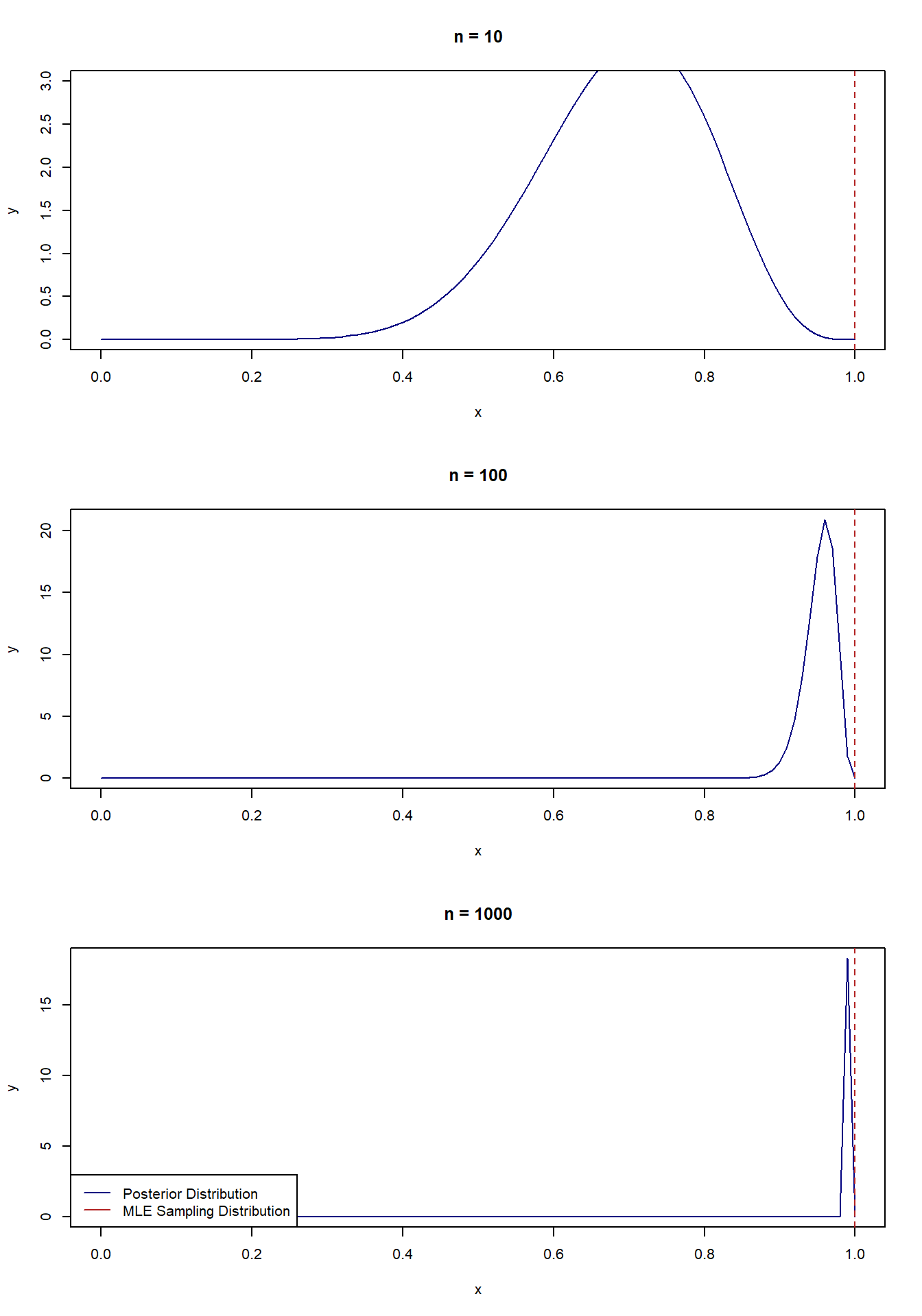
3.3.3 Example 4 - True parameter value is on the boundary
Let’s return to the Bernoulli example from before, but this time we will see what happens when the probability is on the boundary, that is, the true value of \(p = 1\).
Bayesian Approach
Recall the posterior distribution for \(p\) with a \(Beta(1, 5)\) prior is: \[\begin{equation*} p\mid Y_1,\dots, Y_n \sim Beta(1+ \sum_{i=1}^n Y_i, n+5 - \sum_{i=1}^n Y_i) \end{equation*}\]
Frequentist Approach
The MLE \(\hat p = \sum_{i=1}^n Y_i/n\) and the Fisher information is \(1/p(1-p)\). The sampling distribution is then \[\begin{equation*} \hat p \sim N(1, 0). \end{equation*}\]
Note that the variance of the MLE’s sampling distribution is now zero, so in other words, it is just a point mass at \(p=1\)! Let’s see what happens to the posterior.
p_true <- 1

# Functions to calculate the posterior mean and sd
post_alpha <- function(x) {

  1+sum(x)

}

post_beta <- function(x) {

  n <- length(x)

  n+5-sum(x)

}

# Function to calculate asymptotic sd for MLE
mle_sd <- function(p, x) {

  n <- length(x)

  sqrt(p*(1-p)/n)

}

# Generate some data of different sample sizes
set.seed(2022)
y_small <- rbinom(10, size = 1, prob = p_true)
y_med <- rbinom(100, size = 1, prob = p_true)
y_large <- rbinom(1000, size = 1, prob = p_true)

# Set up Plotting
x_vals <- seq(0, 1, by = 0.01)
par(mfrow = c(3,1))

# Plot the asymptotic distribution of MLE and posterior distribution for n  = 10
plot(x_vals, dbeta(x_vals, shape1 = post_alpha(y_small), shape2 = post_beta(y_small)), col = "navy", type = "l",
     ylab = "y", xlab = "x", main = "n = 10", ylim = c(0, 3))
abline(v = p_true, lty = 2, col = "firebrick")

# Plot the asymptotic distribution of MLE and posterior distribution for n  = 50
plot(x_vals, dbeta(x_vals, shape1 = post_alpha(y_med), shape2 = post_beta(y_med)), col = "navy", type = "l",
     ylab = "y", xlab = "x", main = "n = 100")
abline(v = p_true, lty = 2, col = "firebrick")

# Plot the asymptotic distribution of MLE and posterior distribution for n  = 100
plot(x_vals, dbeta(x_vals, shape1 = post_alpha(y_large), shape2 = post_beta(y_large)), col = "navy", type = "l",
     ylab = "y", xlab = "x", main = "n = 1000")
abline(v = p_true, lty = 2, col = "firebrick")
legend("bottomleft", legend = c("Posterior Distribution", "MLE Sampling Distribution"), col = c("navy", "firebrick"), lty = c(1,1))